Journal reading - Self-Organized Criticality: An Explanation of 1/f Noise

Self-Organized Criticality_ An Explanation of 1_f Noise.pdf

자기-조직 임계성: 1/f 노이즈의 원인

이 논문은 2차원 이상의 동역학 시스템이 자기-조직 임계성을 가지는 경우 프랙탈 구조를 갖추게 된다고 이야기한다. 그리고 이 프랙탈 구조에 의해 1/f noise가 나타남을 보였다.

들어가기에 앞서

프랙탈의 멱법칙에 대한 직관적 설명

진동수 성분이 고르게 섞여있으면(백색소음) 너무 무질서
진동수 성분이 한 두개만 특정하게 강하게 나타나면 너무 질서
1/f는 진동수가 적절하게 섞여있거 복잡하다

내용 읽기

One of the classic problems in physics is the existence of the ubiquitous “1/” noise which has been detected for transport in systems as diverse as resistors, the hour glass, the flow of the river Nile, and the luminosity of stars. ’ The low-frequency power spectra of such systems display a power-law behavior over vastly different time scales. Despite much effort, there is no general theory that explains the widespread occurrence of 1/f noise.

1/f noise는 낮은 진동수에서 power spectrum이 1/f를 따르는 특징적인 노이즈를 일컫는다. 이 노이즈를 푸리에 변환해서 다양한 주파수 성분으로 나누면, 낮은 주파수일 수록 이것이 강한 지분을 차지한다.
이상하게 1/f noise가가 많은 현상들에서 관찰된다.
저항에서 흐르는 전류의 노이즈, 모래시계속 모래가 경사면에서 굴러 떨어지는 현상, 나일강의 흐름, 별들의 반짝임 등등.
왜 이렇게 다양한 현상에서 1/f noise가 나타나는지는 아직 밝혀진 바가 없다. 그러나 이 논문에서 한번 가설을 제시해 보겠다.

Another puzzle seeking a physical explanation is the empirical observation that spatially extended objects, including cosmic strings, mountain landscapes, and coastal lines, appear to be self-similar fractal structures. Turbulence is a phenomenon where self-similarity is believed to occur both in time and space. The common feature for all these systems is that the power-law temporal or spatial correlations extend over several decades where naively one might suspect that the physics would vary dramatically.

또 다른 자연 현상에서 풀리지 않는 의문은 다양한 곳에서 자기-유사적 프랙탈(self-similar fractal) 구조가 나타나는 것이다. 우주끈(cosmic string), 산맥의 모양, 해안선등은 모두 자기-유사적 프랙탈을 가진다. 난류(turbulence)는 시간 차원과 공간 차원 모두에서 자기-유사성이 나타나는 것으로 여겨진다. 이런 프랙털 시스템의 공통점은 여러 십진법적 범위(의 단위)에서 power-low의 공간적/시간적 correlation이 발견된다는 것이다.

In this paper, we argue and demonstrate numerically that dynamical systems with extended spatial degrees of freedom naturally evolve into self-organized critical structures of states which are barely stable. We suggest that this self-organized criticality is the common underlying mechanism behind the phenomena described above. The combination of dynamical minimal stability and spatial scaling leads to a power law for temporal fluctuations.

본 논문에서 저자는 확장된 공간 자유도를 가진 동역학 시스템들이 간신히 안정한 상태들의 자기조직화된 임계 구조로 자연스럽게 진화한다는 것을 보여준다. 저자는 이러한 자기조직화 임계성이 1/f noise를 가진 현상들 뒤에 숨겨진 공통의 근본 메커니즘이라고 제안한다. 동역학적 겨우 안정성(dynamical minimal stability)과 공간적 스케일링의 결합은 시간적 변동에 대한 멱법칙(power-low)을 이끈다.

여기서 잠깐, ‘확장된 공간 자유도’란?

공간 위 각 점마다 연속적인 파라미터를 가져서 자유도가 무한한 시스템.
예) 모래시계속 모래더미. xy 평면 위 한 점에서 모래의 높이를 z(x,y)라고 한다면, 상태 공간은 이며, 2차원 공간에 분포된 무한대의 자유도를 가진 것이다.

The noise propagates through the scaling clusters by means of a “domino” effect upsetting the minimally stable states. Long-wavelength perturbations cause a cascade of energy dissipation on all length scales, which is the main characteristic of turbulence.

스케일링 클러스터를 도미노 조각 삼아서, 노이즈는 전파된다. 이 과정에서 시스템은 ‘겨우우 안정적인 상태’(barely stable, minimally stable states)가 된다. 장파장 섭동(perturbation)은 모든 길이 규모에서 에너지 소산(dissipation)의 연쇄반응을 일으키며, 이것이 난류의 주요 특성이다.

여기서 잠깐, 섭동(perturebation)이란?

시스템을 평형 상태에서 벗어나게 하는 작은 교란.
예) 가만히 서있던 오뚜기를 살짝 치기
예) 뒤에서 설명할 줄줄이 진자에서 진자 하나를 톡 치기

여기서 잠깐, 소산(dissipation)이란?

작은 정의로는 에너지가 입자의 미소한 떨림을 일으켜 열에너지로 전환되는 것. 큰 정의로는 비가역 과정에서 에너지가 쓰지 못하는 형태로 소실되는 것.

왜 난류 이야기를 하는가?

커다란 소용돌이(장파장 섭동)이 작은 소용돌이로 쪼개지고, 이게 더 작게 쪼개지면서 결국 물의 열 에너지를 높이기 때문이다.

The criticality in our theory is fundamentally different from the critical point at phase transitions in equilibrium statistical mechanics which can be reached only by tuning of a parameter, for instance the temperature. The critical point in the dynamical systems studied here is an attractor reached by starting far from equilibrium: The scaling properties of the attractor are insensitive to the parameters of the model. This robustness is essential in our explaining that no fine tuning is necessary to generate 1/f noise (and fractal structures) in nature.

이 논문에서 말하는 critical state는 상전이 모델에서 말하는 critical state가 아니다. 상전이의 critical state는, 물이 고체이면서 액체이면서 기체인 게 동시에 일어나는 압력과 온도(삼중점)같이, 시스템의 상태가 바뀌는 특정 파라메터를 의미한다.
이 논문에서 말하는 동역학의 임계 상태는 attractor에 의해 연쇄반응이 일어나서 시스템이 스스로 향하는 흥미로운 상태를 의미한다. 이 흥미로운 상태가 프랙탈이 일어나는 ‘간신히 안정적인 상태’이다. 이 임계 상태는 시스템의 파라메터와 무관하게 일어난다.

‘시스템의 파라메터와 무관하게 일어난다’ 는 게 무슨 말일까?

모래시계와 같은 경우 중력, 모래의 마찰과 같은 요인이 모래더미의 각도에 영향을 끼치지 않는다는 뜻이다. 시스템을 이루는 구성 요소나 사소한 설정이 달라도, 시스템의 ‘확장된 공간적 자유도’가 같은 구성이라면 똑같은 임계 상태에 이른다는 뜻이다.

Consider first a one-dimensional array of damped pendula, with coordinates , connected by torsion springs that are weak compared with the gravitational force. There is an infinity of metastable or stationary states where the pendula are pointing (almost) down, u„ = , N an integer, but where the winding numbers N of the springs differ.

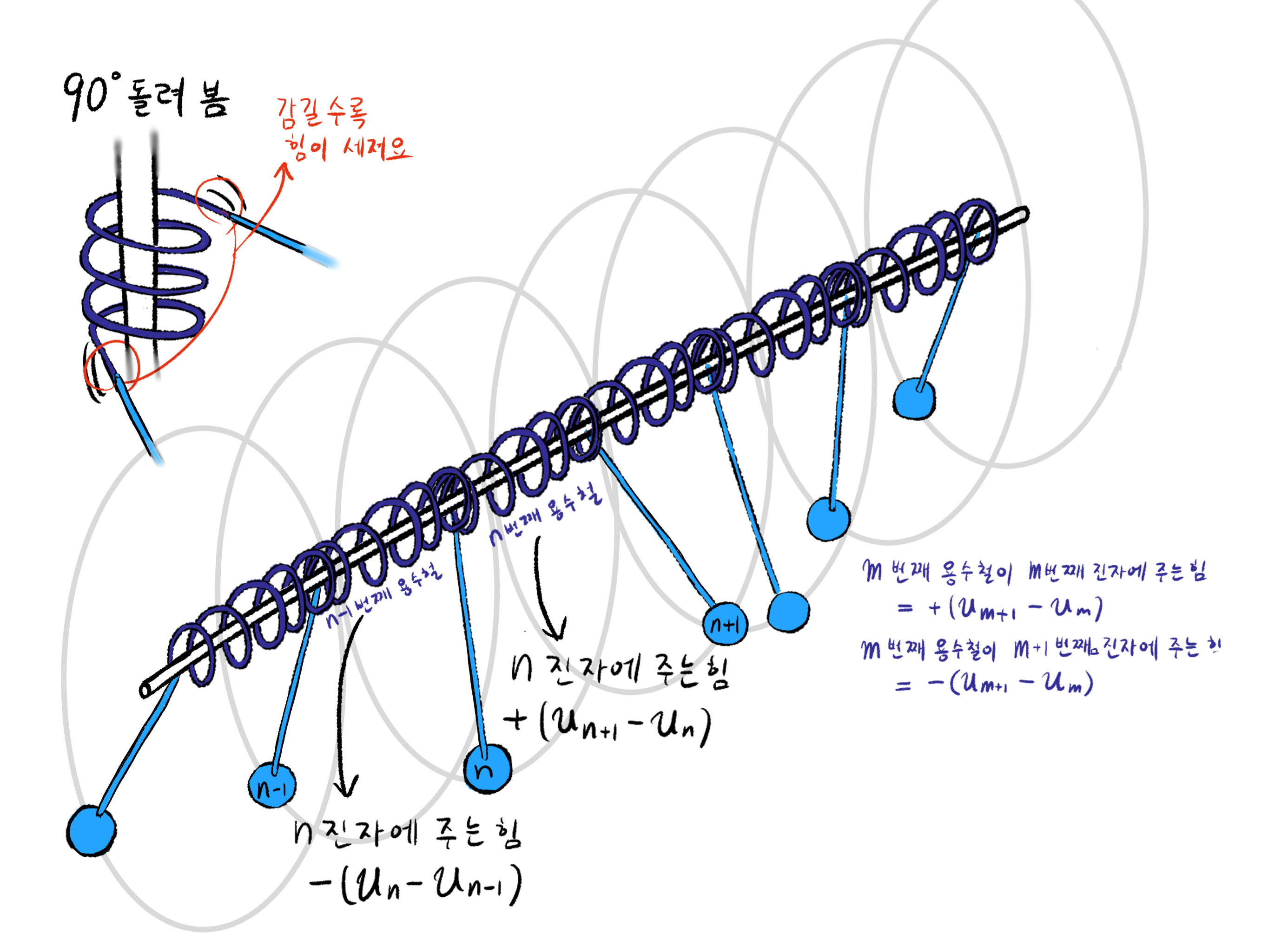
비틀림 용수철로 연결된 줄줄이 진자를 상상해보자. n번째 진자의 각도를 이라고 하자. 비틀림 용수철은 이어진 두 진자의 각도 차이만큼 양쪽에 돌림힘을 준다. 용수철의 힘은 중력보단 약하다. 이 시스템에는 무한대의 준-안정상태와 정지 상태가 있을 것이다. 이 상태에서는 대부분의 진자가 바닥을 향해 있으며, 진자가 돌아간 횟수(용수철이 감긴 횟수?)가 N일 때, 좌표들은 일 것이다.

The initial conditions are such that the forces are large, so that all the pendula are unstable. The pendula will rotate until they reach a state where the spring forces on all the pendula assume a large value + K which is just barely able to balance the gravitational force to keep the configuration stable. If all forces are initially positive, then the final forces will all be K.

n 번째 진자가 양쪽의 용수철로부터 받는 힘의 합이 이다. 으로 주어진다.(그림 참고) 처음 상태(이를테면, 진자의 각도가 무작위로 주어진)에는 용수철 힘이 강하기 때문에 진자들은 불안정할 것이다. 용수철의 힘과 중력이 균형을 이뤄 시스템이 안정적일 때 이라면, 용수철들이 이 힘에 이를 때까지 진자들은 회전할 것이다. 만약 용수철 힘의 초기값이 모두 양수라면, 마지막(시스템이 거의 정지할 때) 용수철 힘은 모두 일 것이다.

Of course, the array is also stable in any configuration where the springs are still further relaxed; however, the dynamics stops upon reaching this first, maximally sensitive state. We call such a state locally minimally stable.

물론, 이 시스템에서 최고로 안정적인 상태는 모든 용수철이 완전히 풀려있고(용수철 힘이 0이고) 진자는 모두 바닥으로 향한 상태일 것이다. 그러나 시스템은 곧바로 이 최대 안정 상태로 가지 않고, 첫번째로 ‘국소적 최소 안정 상태’(locally minimally stable, 이하 겨우 안정 상태)에 머무른다. 가능한 모든 상태에서 최고로 안정적이진 않지만, 인근한 다른 각도를 가진 상태 보다는 제법 안정적인 상태가 ‘겨우 안정 상태’인 것이다. 이곳은 자극에 아주 민감하다. 작은 섭동만으로도 다시 불안정해 질 수 있다.

locally minimally stable을 ‘겨우 안정 상태’로 번역한 이유

원문에서 ‘minimally stable’하다는 건 ‘안정성이 최소’라는 의미이다. 조그만 섭동에도 흔들릴 수 있는 ‘간신히, 겨우 안정적’인 상태라는 뜻이다. 직역하여 ‘최소 안정성’이라고 부르면 마치 에너지가 최소라는 의미로 읽힐 것 같아(국소적으로 에너지가 최소인 건 맞긴 하지만), ‘겨우 안정’이라고 번역했다.

What is the effect of small perturbations on the minimally stable structure? Suppose that we “kick” one pendulum in the forward direction, relaxing the force slightly. This will cause the force on a nearest-neighbor pendulum to exceed the critical value and the perturbation will propagate by a domino effect until it hits the end of the array. At the end of this process the forces are back to their original values, and all pendula have rotated one period. Thus, the system is stable with respect to small perturbations in one dimension and the dynamics is trivial.

겨우 안정 상태에서 약간의 섭동을 일으키면 무슨 일이 생길까? 이어진 용수철의 감김을 푸는 방향으로, 진자 하나를 쳐보자. 이 자극은 용수철을 통해 주변 진자에 까지 영향이 갈 것이고, 진자의 흔들림이 퍼쳐나가기 시작할 것이다. 마치 도미노처럼. 이 진동은 마지막 진자까지 퍼져나갈 것이다. 이 과정을 통해 모든 진자들은 한바퀴를 돌아 다시 원래의 각도로 돌아온다. 모든 진자들이 한바퀴 돌았고, 용수철은 인근 진자의 각도 차이만 보므로, 결과적으로 용수철의 힘은 섭동이 일어나기 이전과 똑같이 모두 이다. 이렇듯, 1차원의 시스템은 겨우 안정 상태태에서 섭동이 일어나도 다시 그 상태로 돌아온다. 이것은 예상 가능한 역학이므로 흥미롭지 않다.

사실, 용수철이 풀리는 방향으로 진자를 밀었을 때 왜 진자가 한 바퀴 돌아야 하는지 이해하지 못 했다.

The situation is dramatically different in more dimensions. Naively, one might expect that the relaxation dynamics will take the system to a configuration where all the pendula are in minimally stable states. A moment’ s reflection will convince us that it cannot be so. Suppose that we relax one pendulum slightly; this will render the surrounding pendula unstable, and the noise will spread to the neighbors in a chain reaction, ever amplifying since the pendula generally are connected with more than two minimally stable pendula, and the perturbation eventually propagates throughout the entire lattice. This configuration is thus unstable with respect to small fluctuations and cannot represent an attracting fixed point for the dynamics.

그러나, 2차원 공간에서는 사정이 극적으로 달라진다. 모든 진자들이 겨우 안정 상태가 되는 것 자체가 불가능하다. 1차원에서는 툭 친 하나의 진자의 양 옆, 두 개의 진자에게만 자극이 전해졌다. 그리고 이 자극은 또 옆의 진자로만 전달되어서, 자극이 도미노처럼 순서대로 일렬로 전해졌다.

2차원에서는 상황이 완전히 다르다. 연결된 4개의 진자에 자극이 동시에 전해진다. 이 경우 자극의 전파가 사방으로 퍼져나가면서 기하급수적으로 증폭될 수 있다. 또한, 1차원에서는 바로 옆의 하나의 진자를 통해서만 자극을 받았지만, 2차원에서는 여러 인근 진자들을 통해 동시에 자극을 전달받을 수도 있어서, 복잡한 간섭과 증폭 현상이 일어난다.

As the system further evolves, more and more more-than-minimally stable states will be generated, and these states will impede the motion of the noise. The system will become stable precisely at the point when the network of minimally stable states has been broken down to the level where the noise signal cannot be communicated through infinite distances At. this point there will be no length scale in the problem so that one might expect the formation of a scale-invariant structure of minimally stable states.

자극 전파가 더 이루어짐에 따라, 간섭 현상에 의해 더 많은 진자들이 ‘겨우 안정보다 더 안정 상태’(more-than-minimally stable, 이하 ‘더 안정 상태’)가 될 것이다. 그리고 이런 진자들은 자극의 전파를 늦출 것이다. 이 진자들은 조금 흔들려도 금방 원래의 ‘더 안정 상태’로 돌아오기 때문이다. 마치, 도미노 행렬 사이에 끼인 벽돌을 생각하면 된다. 가벼운 플라스틱 도미노(겨우 안정 상태 진자)가 넘어져서 벽돌(더 안정 상태 진자)을 툭 쳐도, 벽돌은 거의 흔들리지 않을 것이고, 벽돌 뒤의 도미노는 더 이상 쓰러지지 않을 것이다. 만약 ‘겨우 안정 상태’ 진자가 ‘더 안정 상태’ 진자에 둘러 싸이면, 자극 전파의 방어벽이 생긴 것이고, 자극은 저 이상 무한대로 전파되지 않는다. 이른바 ‘자극 전파의 섬’, ‘겨우 안정 상태 클러스터’가 생기는 것이다. 이 클러스터가 만들어 지는 데에는 정해진 길이 단위가 없다.(scale-invariant structure)

Hence, the system might approach, through a self-organized process, a critical point with power-law correlation functions for noise and other physically observable quantities. The “clusters” of minimally stable states must be defined dynamically as the spatial regions over which a small local perturbation will propagate. In a sense, the dynamically selected configuration is similar to the critical point at a percolation transition where the structure stops carrying current over infinite distances, or at a second-order phase transition where the magnetization clusters stop communicating.

이렇듯, 자기조직화 과정(앞선 사례에서는, 스스로 클러스터를 만드는 과정)을 통해서, 노이즈나 물리량(진자의 각도 )이 멱법칙 상관 함수(power-law correlation functions)를 가지는 임계점에 이른다. 앞서 말한 ‘겨우 안정 상태 클러스터’는 작은 지역적 섭동이 전파될 수 있는 공간적 범위로 정의된다. 어떤 의미에서, 동역학적으로 선택된 이 배치는 percolation 전이의 임계점과 유사하다. 이 점에서는 구조가 무한한 거리에 걸쳐 전류를 전달하는 것을 멈춘다. 또는 자화 클러스터들이 소통을 멈추는 2차 상전이의 임계점과도 유사하다.

여기서 말하는 percolation이 무엇인가?

통계역학에서 유명한 침투 이론(percolation theory)를 의미한다. 흙이 담긴 화분 위에 물을 부었을 때, 과연 물이 바닥까지 침투해 흘러 나올 것인가? 흙이 얼마나 빽빽하게 차 있어야 물이 통과하지 못 할 까? 화분 속 공간을 개의 픽셀로 쪼개 생각하자. 각 픽셀에는 흙 알갱이가 p의 확률로 있거나, p-1의 확률로 없다. 픽셀의 상태는 독립적이다. 흙이 없는 픽셀을 통해서만 물이 흐를 수 있을 테니, 물이 위에서 바닥까지 흐르기 위해서는 흙 없는 빈 공간 클러스터가 화분의 끝에서 끝까지 이어져야 한다.

그러면 수학적으로 질문은 이렇게 정의된다. ‘p값이 얼마가 되어야 경계와 경계를 잇는 빈 공간 클러스터가 확률적으로 생길 수 있을까?’ 물이 흐를 수 있는 빈 공간 클러스터가 존재할 확률 f를 p에 대한 함수로 나타낼 수 있을 것이다.

놀랍게도, 화분이 무한히 크다면(n을 무한대로 보내면) f(p)는 0아니면 1이 된다. 0과 1의 경계를 만드는 임계점을 라고 두자. 인 p에 대해서는 이라서 물이 통과할 수 없고, 인 p에 대해서는 이라서 물이 통과할 수 있다. 인 임계점에서는 빈 공간 클러스터와 흙 클러스터가 적절히 뒤섞여서, 간신히 물이 통하지 않은 상태가 된다.

논문의 내용과 percolation theory를 연관지어 설명해 보자면, 자극이 전파될 수 있는 ‘겨우 안정 상태 클러스터’를 화분에서 물이 흐를 수 있는 ‘빈 공간 클러스터’에 비유할 수 있을 것이다. 2차원 진자의 경우, 임계 상태에서 자극을 무한 거리로 전파할 수 있는 ‘안정 상태 클러스터’가 없으며, 클러스터의 크기에 길이 단위가 없었다. 무한히 큰 화분의 경우에도 임계 상태에서는 간신히 무한한 너비의 빈 공간 클러스터가 없다.

왜 공간적으로 멱법칙 상관 함수(power-law correlation functions)를 가지면 프랙탈 구조라고 말하는 걸까?

이전 포스트를 참고

The arguments are quite general and do not depend on the details of the physical system at hand, including the details of the local dynamics and the presence of impurities, so that one might expect self-similar fractal structures to be widespread in nature: The “physics of fractals” could be that they are the minimally stable states originating from dynamical processes which stop precisely at the critical point.

이런 논증은 상당히 일반적이어서, 국소적 역학이나 불순물등의 자잘한 물리적 세부사항등에 구애받지 않는다. 그러므로 자연 속에서 보편적으로 프랙탈 구조를 찾을 수 있을 거라고 예상할 수 있다. “프랙탈의 물리”는 동역학적 과정에서 ‘겨우 안정 상태’들이 생겨나서 정확히 임계점에서 자기조직(클로스터 형성)이 멈추는 것으로 여겨질 수 있다.

The scaling picture quite naturally gives rise to a power-law frequency dependence of the noise spectrum. At the critical point there is a distribution of clusters of all sizes; local perturbations will therefore propagate over all length scales, leading to fluctuation lifetimes over all time scales. A perturbation can lead to anything from a shift of a single pendulum to an avalanche, depending on where the perturbation is applied. The lack of a characteristic length leads directly to a lack of a characteristic time for the resulting fluctuations.

이러한 크기 성질 덕분에 1/f noise가 생길 수 있다. 임계점에서 모든 크기의 클러스터가 존재하기에, 국소적 섭동이 모든 길이 척도에서 전파될 수 있다. 그리고 섭동이 살아있는(전파되는)시간이 모든 단위의 시간에서 나타난다. 하나의 섭동은 꼴랑 하나의 진자를 흔들리게 할 수도 있으며, 무수한 진자를 흔드는 산사태를 만들 수도 있다. 이 모든 건 섭동이 시작되는 클러스터의 크기에 달렸다. 작은 클러스터이세 시작한 섭동은 짧은 시간 내에 죽을 것이고, 큰 클러스터에서 시작한 섭동은 긴 시간 동안 살아있을 것이다. 이렇듯 공간에서 특성 길이(characteristic length)가 없다면, 노이즈의 시간에서도 특성 시간(characteristic time)이 없어진다.

As is well known, a distribution of lifetimes leads to a frequency spectrum (1) In order to visualize a physical system expected to exhibit self-organized criticality, consider a pile of sand. If the slope is too large, the pile is far from equilibrium, and the pile will collapse until the average slope reaches a critical value where the system is barely stable with respect to small perturbations. The “1/f” noise is the dynamical response of the sandpile to small random perturbations.

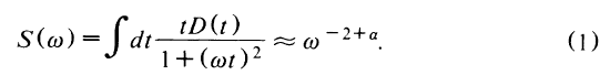
노이즈 수명의 분포가 에 따른다면, frequency spectrum은 (식 1)로 주어진다. 역시, 멱법칙이 유지된다. 특히 a=1이라면, 이어서 1/f noise가 된다는 점에 주목하라.

임계점에서 자기조직하는 시스템의 예시로 모래 더미를 상상해 보라.

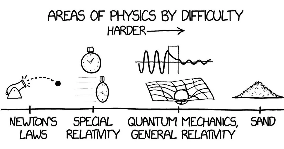
갑자기 이 짤이 생각났다.

모래더미의 경사가 너무 가파르다면, 그 구조는 불안정해서 평형 상태와 멀 것이고, 벽면의 모래는 무너져 떨어져서 적절한 경사가 형성될 때까지 멈추지 않을 것이다. 모래의 굴러떨어짐이 멈출 때면 평균적인 경사는 임계값일 것이다. 이때 모래더미는 거의 안정적이어서, 모래 한 알이 떨어지는 거 같은 작은 섭동이 일어나도 크게 변화하지 않을 것이다. 이 상태의 모래 더미에서, 작은 섭동이 일어나면 1/f noise가 나타난다.

To add concreteness to these considerations we have performed numerical simulations in one, two, and three dimensions on several models, to be described here and in forthcoming papers. One model is a cellular autornaton, describing the interactions of an integer variable with its nearest neighbors. In two dimensions z is updated synchronously as follows:

if z exceeds a critical value K. There are no parameters since a shift in K simply shifts z. Fixed boundary conditions are used, i.e., z =0 on boundaries. The cellular variable may be thought of as the force on an individual pendulum, or the local slope of the sand pile (the “hour glass” ) in some direction. If the force is too large, the pendulum rotates (or the sand slides), relieving the force but increasing the force on the neighbors. The system is set up with random initial conditions z >>K, and then simply evolves until it stops, i.e., all z’s are less than K. The dynamics is then probed by measurement of the response of the resulting state to small local random perturbations. Indeed, we found response on all length scales limited only by the size of the system.

구체적인 수치적 예를 제시하기 위해 우리는 시뮬레이션을 진행했다. 1, 2, 3차원 모두에서 진행했으며, 시스템에서 각 격자점은 z라는 정수값을 가진다. 한 점에서 z가 임계점 K를 넘으면 자기 자신의 z와 이웃들의 값을 수정한다. 2차원 모델의 경우, 값의 수정은 다음과 같이 일어난다.

식 추가

모래더미의 예시로 이해하면 좋다. (x, y) 점에 z개의 모래알이 쌓여 있다고 상상하자. 모래알이 K개 초과로 쌓이면 매우 불안정해져서, 모래알이 1알 씩 상하좌우 사방의 이웃 점으로 이동한다. 결론적으로 (x, y)의 z값은 4 줄어들며, 이웃 , 점들의 z값은 1씩 증가한다.

(x, y)평면의 경계에서는 z=0이 되는 고정된 경계 조건을 사용했다. 시스템이 비평형 상태에서 시작할 때, 모든 z값이 K보다 훨씬 큰 랜덤한 값을 가진다. 시간이 지나면서 모든 z값이 K보다 작은 안정된 상태에 다다를 것이다.

노이즈 값은 이 다음 측정된다. 랜덤한 위치에 작은 섭동을 주어서 그에 대한 반응을 측정한다. 실제로 저자는, 시스템의 사이즈에만 제한되는 모든 길이 척도의 반응을 확인했다.

Figure 1 shows a structure obtained for a two dimensional array of size 100X100. The dark areas indicate clusters that can be reached through the domino process originated by the tripping of only a single site. The clusters are thus defined operationally —in a real physical system one should perturb the system locally in order to measure the size of a cluster. Figure 2(a) shows a log-log plot of the distribution D(s) of cluster sizes for a two-dimensional system determined simply by our counting the number of affected sites generated from a seed at one site and averaging over many arrays. The curve is consistent with a straight line, indicating a power law , . The fact that the curve is linear over two decades indicates that the system is at a critical point with a scaling distribution of clusters.

figure 1은 100x100 격자에서 시뮬레이션한 결과이다. 검은색 영역은 작은 섭동이 전파될 수 있는 ‘겨우 안정 상태’(즉 z값이 K)인 곳이다.

figure 2의 a는 50x50 격자 시스템에서 클러스터 크기 s의 분포 D(s)를 log-log plot으로 그린 것이다. 여러번 격자를 초기화하며 반복 실험한 뒤에 평균낸 것이다. 그래프는 거의 직선을 이루고 있으며, log-log plot에서 직선이 나타난다는 건 멱법칙을 따른다는 뜻이다. 로 근사할 때 로 나타난다.

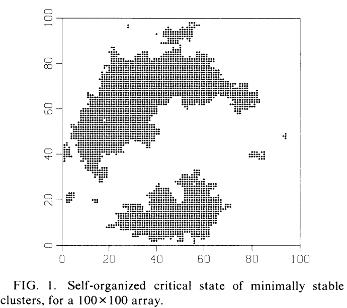
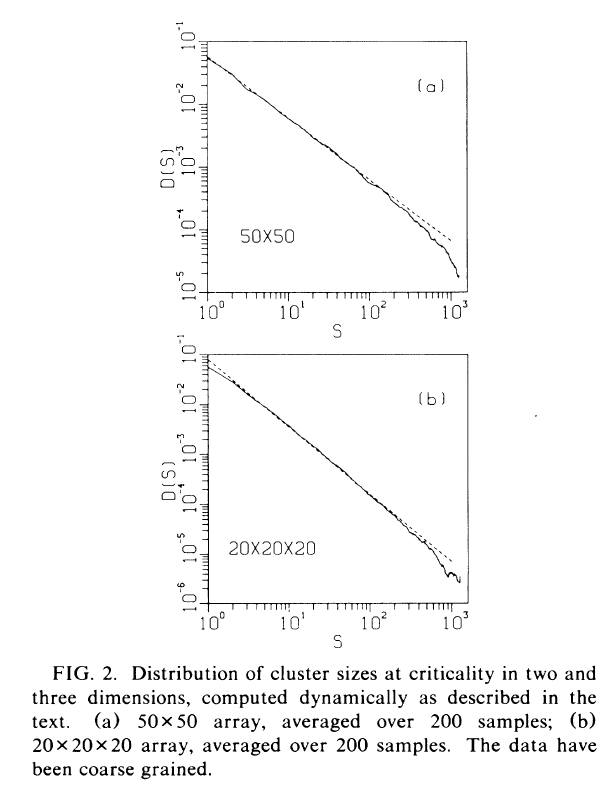
Figure 2(b) shows a similar plot for a three-dimensional array, with an exponent of . At small sizes the curve deviates from the straight line because discreteness effects of the lattice come into play. The falloff at the largest cluster sizes is due to finite-size effects, as we checked by comparing simulations for different array sizes.

figure 2의 b는 3차원의 20x20x20 격자에서 시뮬레이션한 결과이며, 역시 비슷한 형태의 그래프를 보인다. 지수는 이었다. 시스템의 크기가 작아지면서, 격자점의 크기가 반영되므로(이상적인 상태라면 시스템 크기에 비해 격자점이 무한히 작아야 한다) 멱법칙에서 약간 벗어나는 경향을 보인다. (그래프를 보면 직선 점선으로 표시된 것과 실험 값이 조금 차이난다.) 큰 s값에서 D(s)가 갑자기 떨어지는 것은 격자의 크기가 유한하기 때문이다. 이상적으로 무한한 수의 격자가 존재한다면 이런 경향이 보이지 않을 것이다.

A distribution of cluster sizes leads to a distribution of fluctuation lifetimes. If the perturbation grows with an exponent within the clusters, the lifetime t of a cluster is related to its size s by . The distribution of lifetimes, weighted by the average response s/t, can be calculated from the distribution of cluster sizes:

클러스터 크기의 분포는 섭동의 수명 분포로 이어진다. 만약 섭동이 전파되는 격자점이 클러스터 내부에서 지수 함수로 성장한다면(지수가 일 때), 섭동의 수명 t는 클러스터의 크기 s와 의 관계를 가진다. 그래서 섭동 수명의 분포 D(t)는 아래 식으로 주어진다.

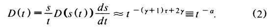
어떻게 이 식이 유도되는 건지 모르겠다! 특히 ‘섭동의 수명 t는 클러스터의 크기 s와 의 관계’ 에서 왜 tau가 나왔는지 모르겠다. t를 잘못 쓴 건가? 이게 오타가 맞다면 비로소 식 2가 이해된다.

Figure 3 shows the distribution of lifetimes corresponding to Fig. 2 (namely how long the noise propagates after perturbation at a single site, weighted by the temporal average of the response). This leads to another line indicating a distribution of lifetimes of the form (2) with in two dimensions (50X50), and in three dimensions. These curves are less impressive than the corresponding cluster-size curves, in particular in three dimensions, because the lifetime of a cluster is much smaller than its size, reducing the range over which we have reliable data. The resulting power-law spectrum is in 2D and in 3D.

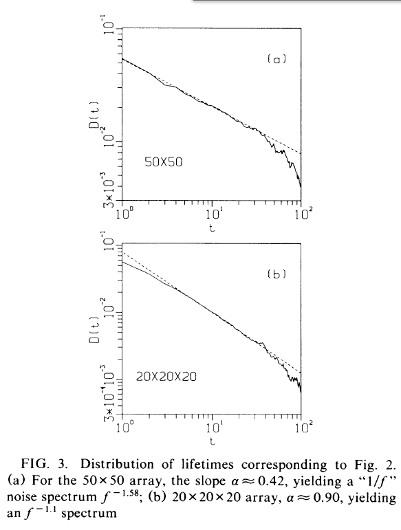
Figure 3은 Figure 2에 대응하는 수명 분포를 보여준다 (즉, 단일 지점에서 섭동 이후 노이즈가 얼마나 오래 전파되는지를, 응답의 시간 평균으로 가중하여 나타낸 것). 이는 식 (2) 형태의 수명 분포를 나타내는 또 다른 직선을 보여주며, 2차원(50x50)에서는 3차원에서는 이다. 이 곡선들은 대응하는 클러스터 크기 곡선들보다 덜 인상적인데, 특히 3차원에서 그러하다. 그 이유는 클러스터의 수명이 그 크기보다 훨씬 작아서, 신뢰할 수 있는 데이터를 얻을 수 있는 범위가 줄어들기 때문이다. 결과적인 멱법칙 스펙트럼은 2차원에서 이고, 3차원에서는 이다.

To summarize, we find a power-law distribution of cluster sizes and time scales just as expected from general arguments about dynamical systems with spatial degrees of freedom. More numerical work is clearly needed to improve accuracy, and to determine the extent to which the systems are “universal, ” e.g., how’ the exponents depend on the physical details. Our picture of 1/f spectra is that it reflects the dynamics of a selforganized critical state of minimally stable clusters of all length scales, which in turn generates fluctuations on all time scales.

요약하자면, 우리는 공간 자유도를 가진 동역학 시스템에 대한 일반적 논증으로부터 예상했던 것처럼, 클러스터 크기와 시간 척도의 멱법칙 분포를 발견했다. 정확도를 높이고 시스템이 어느 정도까지 “보편적”인지 - 예를 들어, 지수들이 물리적 세부사항에 어떻게 의존하는지 - 를 결정하기 위해서는 더 많은 수치 연구가 분명히 필요하다. 1/f 스펙트럼에 대한 우리의 그림은, 이것이 모든 길이 척도의 겨우 안정한 클러스터들로 이루어진 자기조직화된 임계 상태의 동역학을 반영하며, 이것이 다시 모든 시간 척도에서의 변동을 생성한다는 것이다.